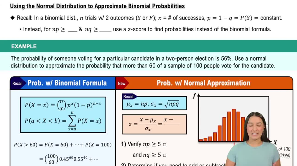
Afraid to Fly According to a study conducted by the Gallup organization, the proportion of Americans who are afraid to fly is 0.10. A random sample of 1100 Americans results in 121 indicating that they are afraid to fly. Explain why this is not necessarily evidence that the proportion of Americans who are afraid to fly has increased since the time of the Gallup study.
Table of contents
- 1. Intro to Stats and Collecting Data1h 14m
- 2. Describing Data with Tables and Graphs1h 55m
- 3. Describing Data Numerically2h 5m
- 4. Probability2h 16m
- 5. Binomial Distribution & Discrete Random Variables3h 6m
- 6. Normal Distribution and Continuous Random Variables2h 11m
- 7. Sampling Distributions & Confidence Intervals: Mean3h 23m
- Sampling Distribution of the Sample Mean and Central Limit Theorem19m
- Distribution of Sample Mean - Excel23m
- Introduction to Confidence Intervals15m
- Confidence Intervals for Population Mean1h 18m
- Determining the Minimum Sample Size Required12m
- Finding Probabilities and T Critical Values - Excel28m
- Confidence Intervals for Population Means - Excel25m
- 8. Sampling Distributions & Confidence Intervals: Proportion1h 25m
- 9. Hypothesis Testing for One Sample3h 29m
- 10. Hypothesis Testing for Two Samples4h 50m
- Two Proportions1h 13m
- Two Proportions Hypothesis Test - Excel28m
- Two Means - Unknown, Unequal Variance1h 3m
- Two Means - Unknown Variances Hypothesis Test - Excel12m
- Two Means - Unknown, Equal Variance15m
- Two Means - Unknown, Equal Variances Hypothesis Test - Excel9m
- Two Means - Known Variance12m
- Two Means - Sigma Known Hypothesis Test - Excel21m
- Two Means - Matched Pairs (Dependent Samples)42m
- Matched Pairs Hypothesis Test - Excel12m
- 11. Correlation1h 24m
- 12. Regression1h 50m
- 13. Chi-Square Tests & Goodness of Fit2h 21m
- 14. ANOVA1h 57m
8. Sampling Distributions & Confidence Intervals: Proportion
Sampling Distribution of Sample Proportion
Problem 8.2.5
Textbook Question
Describe the circumstances under which the shape of the sampling distribution of p̂ is approximately normal.
Verified step by step guidance1
Understand that \( \hat{p} \) represents the sample proportion, which is a random variable based on the outcomes of a sample from a population.
Recall that the sampling distribution of \( \hat{p} \) describes the distribution of sample proportions over many repeated samples of the same size from the population.
The shape of the sampling distribution of \( \hat{p} \) is approximately normal when the sample size \( n \) is sufficiently large, and the population proportion \( p \) is not too close to 0 or 1.
Specifically, the normal approximation is appropriate if both \( n \times p \geq 10 \) and \( n \times (1 - p) \geq 10 \). These conditions ensure that there are enough expected successes and failures in the sample for the distribution to be symmetric and bell-shaped.
When these conditions are met, the Central Limit Theorem applies, and the sampling distribution of \( \hat{p} \) can be approximated by a normal distribution with mean \( p \) and standard deviation \( \sqrt{\frac{p(1-p)}{n}} \).
Verified video answer for a similar problem:This video solution was recommended by our tutors as helpful for the problem above
Video duration:
1mPlay a video:
Was this helpful?
Key Concepts
Here are the essential concepts you must grasp in order to answer the question correctly.
Sampling Distribution of p̂
The sampling distribution of p̂ refers to the probability distribution of the sample proportion calculated from repeated random samples of the same size from a population. It shows how p̂ varies from sample to sample and is fundamental for making inferences about the population proportion.
Recommended video:
Sampling Distribution of Sample Proportion
Normal Approximation to the Sampling Distribution
The sampling distribution of p̂ is approximately normal when the sample size is large enough, allowing the Central Limit Theorem to apply. This means the distribution of p̂ will be symmetric and bell-shaped, enabling the use of normal probability methods for inference.
Recommended video:
Using the Normal Distribution to Approximate Binomial Probabilities
Conditions for Normality: np and n(1-p)
For the sampling distribution of p̂ to be approximately normal, both np and n(1-p) must be at least 10, where n is the sample size and p is the population proportion. This ensures enough expected successes and failures to justify the normal approximation.
Recommended video:
Guided course
Z-Scores from Probabilities
Watch next
Master Using the Normal Distribution to Approximate Binomial Probabilities with a bite sized video explanation from Patrick
Start learningRelated Videos
Related Practice
Textbook Question
51
views
