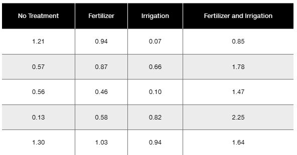
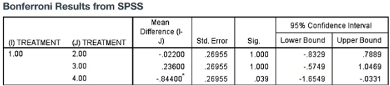
Weights from ANSUR I and ANSUR II The following table lists weights (kg) of randomly selected U.S. Army personnel obtained from the ANSUR I study conducted in 1988 and the ANSUR II study conducted in 2012. If we use the data with two-way analysis of variance and a 0.05 significance level, we get the accompanying display. What do you conclude?
Table of contents
- 1. Intro to Stats and Collecting Data1h 14m
- 2. Describing Data with Tables and Graphs1h 55m
- 3. Describing Data Numerically2h 5m
- 4. Probability2h 16m
- 5. Binomial Distribution & Discrete Random Variables3h 6m
- 6. Normal Distribution and Continuous Random Variables2h 11m
- 7. Sampling Distributions & Confidence Intervals: Mean3h 23m
- Sampling Distribution of the Sample Mean and Central Limit Theorem19m
- Distribution of Sample Mean - Excel23m
- Introduction to Confidence Intervals15m
- Confidence Intervals for Population Mean1h 18m
- Determining the Minimum Sample Size Required12m
- Finding Probabilities and T Critical Values - Excel28m
- Confidence Intervals for Population Means - Excel25m
- 8. Sampling Distributions & Confidence Intervals: Proportion2h 10m
- 9. Hypothesis Testing for One Sample5h 9m
- Steps in Hypothesis Testing1h 6m
- Performing Hypothesis Tests: Means1h 4m
- Hypothesis Testing: Means - Excel42m
- Performing Hypothesis Tests: Proportions37m
- Hypothesis Testing: Proportions - Excel27m
- Performing Hypothesis Tests: Variance12m
- Critical Values and Rejection Regions28m
- Link Between Confidence Intervals and Hypothesis Testing12m
- Type I & Type II Errors17m
- 10. Hypothesis Testing for Two Samples5h 37m
- Two Proportions1h 13m
- Two Proportions Hypothesis Test - Excel28m
- Two Means - Unknown, Unequal Variance1h 3m
- Two Means - Unknown Variances Hypothesis Test - Excel12m
- Two Means - Unknown, Equal Variance15m
- Two Means - Unknown, Equal Variances Hypothesis Test - Excel9m
- Two Means - Known Variance12m
- Two Means - Sigma Known Hypothesis Test - Excel21m
- Two Means - Matched Pairs (Dependent Samples)42m
- Matched Pairs Hypothesis Test - Excel12m
- Two Variances and F Distribution29m
- Two Variances - Graphing Calculator16m
- 11. Correlation1h 24m
- 12. Regression3h 33m
- Linear Regression & Least Squares Method26m
- Residuals12m
- Coefficient of Determination12m
- Regression Line Equation and Coefficient of Determination - Excel8m
- Finding Residuals and Creating Residual Plots - Excel11m
- Inferences for Slope31m
- Enabling Data Analysis Toolpak1m
- Regression Readout of the Data Analysis Toolpak - Excel21m
- Prediction Intervals13m
- Prediction Intervals - Excel19m
- Multiple Regression - Excel29m
- Quadratic Regression15m
- Quadratic Regression - Excel10m
- 13. Chi-Square Tests & Goodness of Fit2h 21m
- 14. ANOVA2h 28m
14. ANOVA
Two-Way ANOVA
Problem 12.1.18b
Textbook Question
Bonferroni Test Shown below are weights (kg) of poplar trees obtained from trees planted in a rich and moist region. The trees were given different treatments identified in the table below. The data are from a study conducted by researchers at Pennsylvania State University and were provided by Minitab, Inc. Also shown are partial results from using the Bonferroni test with the sample data.

b. What do the displayed Bonferroni SPSS results tell us?

Verified step by step guidance1
Step 1: Understand the context of the Bonferroni test. It is a post-hoc multiple comparison test used after an ANOVA to determine which specific group means are significantly different from each other while controlling the overall Type I error rate.
Step 2: Identify the treatments being compared. The treatments are No Treatment (1), Fertilizer (2), Irrigation (3), and Fertilizer and Irrigation (4). The Bonferroni results table compares the mean differences between No Treatment (1) and each of the other treatments.
Step 3: Interpret the 'Mean Difference (I-J)' column. This shows the difference in average weights between the No Treatment group and each other treatment group. For example, the difference between No Treatment and Fertilizer is -0.02200, indicating the Fertilizer group has a slightly lower mean weight than No Treatment.
Step 4: Look at the 'Sig.' (significance) column to determine if the differences are statistically significant. A value less than the chosen alpha level (commonly 0.05) indicates a significant difference. Here, the significance values for comparisons with Fertilizer and Irrigation are 1.000 and 0.393 respectively, which are not significant, but the comparison with Fertilizer and Irrigation combined is 0.039, which is significant.
Step 5: Examine the 95% confidence intervals for the mean differences. If the interval includes zero, it suggests no significant difference. For the Fertilizer and Irrigation combined treatment, the confidence interval does not include zero (-1.6549 to -0.0331), confirming the significant difference found in the significance column.
Verified video answer for a similar problem:This video solution was recommended by our tutors as helpful for the problem above
Video duration:
4mPlay a video:
Was this helpful?
Key Concepts
Here are the essential concepts you must grasp in order to answer the question correctly.
Bonferroni Test
The Bonferroni test is a multiple comparison procedure used after an ANOVA to control the overall Type I error rate when making pairwise comparisons. It adjusts the significance level by dividing it by the number of comparisons, making it more stringent to declare differences significant. This helps prevent false positives when testing multiple hypotheses simultaneously.
Recommended video:
Guided course
Independence Test
Interpretation of SPSS Bonferroni Output
The SPSS Bonferroni output shows pairwise mean differences between treatment groups, their standard errors, significance values (p-values), and confidence intervals. A significant p-value (typically < 0.05) indicates a statistically significant difference between the two treatment means. Confidence intervals that do not include zero also support significant differences.
Recommended video:
Empirical Rule of Standard Deviation and Range Rule of Thumb
Multiple Comparisons in Experimental Design
In experiments with multiple treatment groups, multiple comparisons are necessary to identify which groups differ. However, conducting many tests increases the chance of Type I errors. Methods like the Bonferroni correction adjust for this by controlling the family-wise error rate, ensuring that the overall probability of making one or more false discoveries remains low.
Recommended video:
Tukey Test
Watch next
Master Intro to Two-Way ANOVA & Two-Way Tables with a bite sized video explanation from Patrick
Start learningRelated Videos
Related Practice
Textbook Question
5
views
