
Textbook Question
"Finding a Critical F-Value for a Right-Tailed Test In Exercises 5–8, find the critical F-value for a right-tailed test using the level of significance α and degrees of freedom d.f.N and d.f.D.
α=0.025, d.f.N=7, d.f.D=3"
70
views

 Verified step by step guidance
 06:28
06:28
 05:50
05:50 05:52
05:52"Finding a Critical F-Value for a Right-Tailed Test In Exercises 5–8, find the critical F-value for a right-tailed test using the level of significance α and degrees of freedom d.f.N and d.f.D.
α=0.025, d.f.N=7, d.f.D=3"
Performing a Two-Sample F-Test In Exercises 19–26, (a) identify the claim and state H0 and Ha, (b) find the critical value and identify the rejection region, (c) find the test statistic F, (d) decide whether to reject or fail to reject the null hypothesis, and (e) interpret the decision in the context of the original claim. Assume the samples are random and independent, and the populations are normally distributed.
Heart Transplant Waiting Times The table at the left shows a sample of the waiting times (in days) for a heart transplant for two age groups. At α=0.05, can you conclude that the variances of the waiting times differ between the two age groups? (Adapted from Organ Procurement and Transplantation Network)
Finding Expected Frequencies
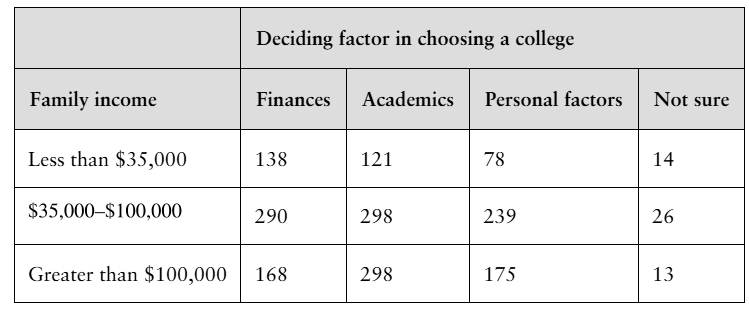
In Exercises 7–12, (a) calculate the marginal frequencies and (b) find the expected frequency for each cell in the contingency table. Assume that the variables are independent.
Testing for Normality Using a chi-square goodness-of-fit test, you can decide, with some degree of certainty, whether a variable is normally distributed. In all chi-square tests for normality, the null and alternative hypotheses are as listed below.
H₀: The variable has a normal distribution.
Hₐ: The variable does not have a normal distribution.
To determine the expected frequencies when performing a chi-square test for normality, first estimate the mean and standard deviation of the frequency distribution. Then, use the mean and standard deviation to compute the z-score for each class boundary. Then, use the z-scores to calculate the area under the standard normal curve for each class. Multiplying the resulting class areas by the sample size yields the expected frequency for each class.In Exercises 17 and 18, (a) find the expected frequencies, (b) find the critical value and identify the rejection region, (c) find the chi-square test statistic, (d) decide whether to reject or fail to reject the null hypothesis, and (e) interpret the decision in the context of the original claim.
In Exercises 17 and 18, (a) find the expected frequencies, (b) find the critical value and identify the rejection region, (c) find the chi-square test statistic, (d) decide whether to reject or fail to reject the null hypothesis, and (e) interpret the decision in the context of the original claim.
Test Scores At α=0.05, test the claim that the 400 test scores shown in the frequency distribution are normally distributed.
Performing a Chi-Square Goodness-of-Fit Test
In Exercises 7–16, (a) identify the claim and state H₀ and Hₐ, (b) find the critical value and identify the rejection region, (c) find the chi-square test statistic, (d) decide whether to reject or fail to reject the null hypothesis, and (e) interpret the decision in the context of the original claim.
Homicides by Month A researcher claims that the number of homicide crimes in California by month is uniformly distributed. To test this claim, you randomly select 2000 homicides from a recent year and record the month when each happened. The table shows the results. At α=0.10, test the researcher’s claim. (Adapted from California Department of Justice)
In each exercise,
d. decide whether to reject or fail to reject the null hypothesis, and
e. interpret the decision in the context of the original claim.
In Exercises 1 and 2, use the table, which lists the distribution of educational achievement for people in the United States ages 25 and older. It also lists the results of a random survey for two additional age groups. (Adapted from U.S. Census Bureau)
Use the data for 30- to 34-year-olds and 65- to 69-year-olds to test whether age and educational attainment are related. Use α=0.01.