Ch. 9 - Inferences from Two Samples

Triola - Elementary Statistics 14th Edition

Triola14th EditionElementary StatisticsISBN: 9780137366446Not the one you use?Change textbook

Triola 14th Edition

Ch. 9 - Inferences from Two Samples

Problem 9.2.5b

Chapter 9, Problem 9.2.5b

In Exercises 5–20, assume that the two samples are independent simple random samples selected from normally distributed populations, and do not assume that the population standard deviations are equal. (Note: Answers in Appendix D include technology answers based on Formula 9-1 along with “Table” answers based on Table A-3 with df equal to the smaller of n1-1 and n2-1)

Better Tips by Giving Candy An experiment was conducted to determine whether giving candy to dining parties resulted in greater tips. The mean tip percentages and standard deviations are given below along with the sample sizes (based on data from “Sweetening the Till: The Use of Candy to Increase Restaurant Tipping,” by Strohmetz et al., Journal of Applied Social Psychology, Vol. 32, No. 2).

b. Construct the confidence interval suitable for testing the claim in part (a).

Verified step by step guidance

Step 1: Identify the given data for both groups. For the 'No Candy' group: sample size (n₁) = 20, mean (x̄₁) = 18.95, standard deviation (s₁) = 1.50. For the 'Two Candies' group: sample size (n₂) = 20, mean (x̄₂) = 21.62, standard deviation (s₂) = 2.51.

Step 2: Use the formula for the confidence interval for the difference between two means when the population standard deviations are not assumed to be equal. The formula is: CI = (x̄₁ - x̄₂) ± t * √((s₁²/n₁) + (s₂²/n₂)), where t is the critical value from the t-distribution table based on degrees of freedom (df).

Step 3: Calculate the degrees of freedom (df) using the formula: df = ((s₁²/n₁ + s₂²/n₂)²) / (((s₁²/n₁)² / (n₁ - 1)) + ((s₂²/n₂)² / (n₂ - 1))). This will determine the appropriate t-value for the confidence interval.

Step 4: Find the critical t-value corresponding to the desired confidence level (e.g., 95%) and the calculated degrees of freedom. Use a t-distribution table or technology to find this value.

Step 5: Substitute the values for x̄₁, x̄₂, s₁, s₂, n₁, n₂, and the critical t-value into the confidence interval formula to compute the interval. Interpret the interval in the context of the problem to determine whether giving candy results in greater tips.

Verified video answer for a similar problem:

This video solution was recommended by our tutors as helpful for the problem above.

Video duration:

Was this helpful?

Key Concepts

Here are the essential concepts you must grasp in order to answer the question correctly.

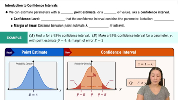
Confidence Interval

A confidence interval is a range of values, derived from sample statistics, that is likely to contain the true population parameter. It is calculated using the sample mean, standard deviation, and sample size, along with a critical value from the t-distribution or z-distribution, depending on the sample size and whether the population standard deviation is known. In this context, constructing a confidence interval will help assess the difference in tip percentages between the two groups.

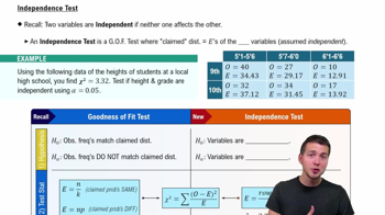
Independent Samples

Independent samples refer to two or more groups that are not related or paired in any way. In this experiment, the tips from dining parties that received candy are independent of those that did not. This independence is crucial for applying statistical tests, as it ensures that the results from one sample do not influence the results from another, allowing for valid comparisons between the groups.

T-test for Independent Samples

A t-test for independent samples is a statistical method used to determine if there is a significant difference between the means of two independent groups. It is particularly useful when the population standard deviations are unknown and the sample sizes are small. In this case, the t-test will help evaluate whether the difference in mean tip percentages between the groups (with and without candy) is statistically significant.

Recommended video:

Guided course

06:28

Independence Test

Related Practice

Textbook Question

Count Five Test for Comparing Variation in Two Populations Repeat Exercise 16 “Blanking Out on Tests,” but instead of using the F test, use the following procedure for the “count five” test of equal variations (which is not as complicated as it might appear).

b. Let c1 be the count of the number of absolute deviation values in the first sample that are greater than the largest absolute deviation value in the other sample. Also, let C2 be the count of the number of absolute deviation values in the second sample that are greater than the largest absolute deviation value in the other sample. (One of these counts will always be zero.)

views

Textbook Question

In Exercises 5–16, use the listed paired sample data, and assume that the samples are simple random samples and that the differences have a distribution that is approximately normal.

Measured and Reported Weights Listed below are measured and reported weights (lb) of random female subjects (from Data Set 4 “Measured and Reported” in Appendix B).

b. Construct the confidence interval that could be used for the hypothesis test described in part (a). What feature of the confidence interval leads to the same conclusion reached in part (a)?

121

views

Textbook Question

In Exercises 5–16, use the listed paired sample data, and assume that the samples are simple random samples and that the differences have a distribution that is approximately normal.

Do Men Talk Less than Women? Listed below are word counts of males and females in couple relationships (from Data Set 14 “Word Counts” in Appendix B).

b. Construct the confidence interval that could be used for the hypothesis test described in part (a). What feature of the confidence interval leads to the same conclusion reached in part (a)?

112

views

Textbook Question

In Exercises 5–20, assume that the two samples are independent simple random samples selected from normally distributed populations, and do not assume that the population standard deviations are equal. (Note: Answers in Appendix D include technology answers based on Formula 9-1 along with “Table” answers based on Table A-3 with df equal to the smaller of n1-1 and n2-1)

Queues Listed on the next page are waiting times (seconds) of observed cars at a Delaware inspection station. The data from two waiting lines are real observations, and the data from the single waiting line are modeled from those real observations. These data are from Data Set 30 “Queues” in Appendix B. The data were collected by the author.

b. Construct the confidence interval suitable for testing the claim in part (a).

100

views

Textbook Question

Readability of Font On a Computer Screen The statistics shown below were obtained from a standard test of readability of fonts on a computer screen (based on data from “Reading on the Computer Screen: Does Font Type Have Effects on Web Text Readability?” by Ali et al., International Education Studies, Vol. 6, No. 3). Reading speed and accuracy were combined into a readability performance score (x), where a higher score represents better font readability.

b. Construct the confidence interval suitable for testing the claim in part (a).

106

views

Textbook Question

Bicycle Commuting A researcher used two different bicycles to commute to work. One bicycle was steel and weighed 30.0 lb; the other was carbon and weighed 20.9 lb. The commuting times (minutes) were recorded with the results shown below (based on data from “Bicycle Weights and Commuting Time,” by Jeremy Groves, British Medical Journal).

b. Construct the confidence interval suitable for testing the claim in part (a).

107

views