In each exercise,
d. decide whether to reject or fail to reject the null hypothesis, and
e. interpret the decision in the context of the original claim.


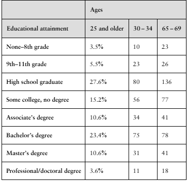
In Exercises 1 and 2, use the table, which lists the distribution of educational achievement for people in the United States ages 25 and older. It also lists the results of a random survey for two additional age groups. (Adapted from U.S. Census Bureau)





Use the data for 30- to 34-year-olds and 65- to 69-year-olds to test whether age and educational attainment are related. Use α=0.01.

Verified step by step guidance

1. Step 1: Define the null hypothesis (H₀) and the alternative hypothesis (H₁). The null hypothesis states that age and educational attainment are not related (independent). The alternative hypothesis states that age and educational attainment are related (dependent).
2. Step 2: Choose the significance level (α). In this case, α = 0.01, which means there is a 1% risk of rejecting the null hypothesis when it is true.
3. Step 3: Organize the data into a contingency table. Use the provided table to structure the observed frequencies for the two age groups (30–34 and 65–69) across the educational attainment categories.
4. Step 4: Calculate the expected frequencies for each cell in the contingency table. Use the formula: E = (row total × column total) / grand total, where E represents the expected frequency for a cell.
5. Step 5: Perform a chi-square test for independence. Compute the test statistic using the formula: χ² = Σ((O - E)² / E), where O is the observed frequency and E is the expected frequency. Compare the calculated χ² value to the critical value from the chi-square distribution table at α = 0.01 with the appropriate degrees of freedom (df = (number of rows - 1) × (number of columns - 1)). Decide whether to reject or fail to reject the null hypothesis based on this comparison.

Key Concepts

Null Hypothesis

The null hypothesis is a statement that there is no effect or no difference, and it serves as a starting point for statistical testing. In this context, it would assert that there is no relationship between age and educational attainment. Researchers aim to gather evidence to either reject or fail to reject this hypothesis based on the data collected.

Significance Level (α)

The significance level, denoted as α, is the threshold for determining whether to reject the null hypothesis. In this case, α is set at 0.01, meaning there is a 1% risk of concluding that a relationship exists when there is none. This stringent level indicates a strong requirement for evidence before rejecting the null hypothesis.

Chi-Square Test

The Chi-Square test is a statistical method used to determine if there is a significant association between categorical variables. In this scenario, it will be applied to assess whether age groups (30-34 and 65-69) are related to different levels of educational attainment. The test compares observed frequencies in each category to expected frequencies under the null hypothesis.