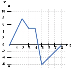
Pearson+ LogoPearson+ Logo
Start typing, then use the up and down arrows to select an option from the list.

Physics

Learn the toughest concepts covered in Physics with step-by-step video tutorials and practice problems by world-class tutors

Table of contents
2. 1D Motion / Kinematics

Position-Time Graphs & Velocity

1
concept

Intro to Position-Time Graphs & Velocity

clock
7m
Play a video:
Was this helpful?
Hey, guys. So sometimes in your problems you're gonna be given graphs instead of numbers. So in this video, we're to talk about position time graphs and how we use them to calculate things like velocity. Let's check it out now, guys, the basic idea is that a position time graph just shows Ewan objects position in the Y axis. So right here versus time inthe e x axis over here. So right off the bat, That might be kind of confusing because we're gonna use position, which is given by the variable X, but it's actually in the Y axis or the vertical axis. So don't let that confuse you. Make sure you understand that. Now what position time graphs do is they help us sort of understand or visualized the motion of an object much more simply, for example, let's say you wanna walk 6 m forward in three seconds, you stop and then you run 6 m back. So you have to basically draw all the points A B, C D. Label, all the parts and things like that. So we can do is we can actually take this complicated diagram. We could actually represent it much more simply on this graph Here, for example, if you were to go 6 m forward in three seconds on the position time graph, you're going from zero all the way up to six and then in three seconds. So you basically just go up and over six and then three. So you're gonna end up right over here, and then we just connect where you started, from which is at the origin and with just with a straight line like this now, finally are. The second part is that you could have stopped for one second. So basically, from B to C, you actually haven't moved anywhere. It's hard to see on the diagram what's actually happening. But from 3 to 4, if you're not moving anywhere, then your position just stays the same. You started six and you stay at six. So that means we're just gonna connect these points with a straight line. And then finally, you're gonna go from four seconds all the way back to five. And so that just means from 4 to 5 over here, you're going all the way back to where you started from, so that we can label the pieces here A B C indeed. So this graph here just represents everything you did on this diagram, but all kind of just in one place without having to draw all these little things here. And it kind of looks weird. So what The position time graphs also dio is we can calculate the velocity directly from the graph. For example, we know that the the equation is Delta X over Delta T. So, for instance, if I look at the interval from A to B, this little line here, I can actually break this up into a triangle, and I can take a look at the legs of the triangle the legs of this triangle. The vertical piece over here actually represents my change in position because that's on the vertical axis. So you can think about this as like the rise of the graph and the horizontal section, the horizontal leg is delta T. That's the change in time. And you can think about this as the run of the graph. So that means that my Delta X over Delta t on this graph is really just the rise over the run. And that's a phrase we've seen before. it's the slope. So, guys, the velocity is the slope of the position graph. And there's a couple things you wanna know when you have upward slopes like we did from A to B. That just means that you're moving forward. And that makes sense because that represents this motion. Here we move forward. If you have a horizontal slope basically a flat one like this, then that means that you stopped because your position isn't changing. And then finally, a downward slope like this from C to D is when you're moving backwards. Like just We were like Like we're moving in that last section over here, guys, that's all you need to know. Basically, there's just one simple equation. We're looking at a bunch of slopes, calculating some slopes. So let's just get to an example. So you've got this position time graph here. I'm going to calculate the average velocities for these parts. Let's check it out. So we're gonna go from 0 to 2 seconds. All you have to do is just go from 0 to 2, and we just need to identify those points on the graph. So zero, I'm over here and it's too I'm over here and I'm just gonna calculate the slope of this line. So let's go ahead and do that. My average velocity is just Delta X over Delta T. So on the graph, I'm gonna go. I'm gonna I'm gonna end to 10. But I'm gonna start at negative 10. So that means that the Delta X is my final position, which is 10 minus my initial position, which is negative. 10. So this is my final Sorry. That's my initial. That's my final. And so my Delta X is just equal to 20. So I've got 20 and then the time is just from 0 to 2 seconds, so that's just too So that means just to get a positive 10 m per second for the velocity here. All right, let's move on. So the second part is gonna be from T equals two t equals for same thing. We're just gonna go from t equals to two t equals for the lines already drawn for us. Now we just have to calculate the slope. So my average velocity here is just gonna be Delta X over Delta T. So what's the rise? Well, if you notice here we've got a flat line. So that means that the rises zero you actually haven't moved anywhere. You started off a 10 and you ended up a 10. So you haven't actually moved anywhere. There's no rise. So that means that zero over. Whatever the time is in this case, Delta T equals two seconds Doesn't matter because you're still gonna end up with a velocity of zero. And that makes sense because 0 m per second means that you should have a horizontal or a flat slope like this on Ben. You know, when we got 10 m per second, we actually just got an upward slopes. That also makes sense. Now, for the last one, Teak was 4 to 5. So this is just gonna be this section right here from T equals 45 So my Delta X, my rise is gonna be while I'm going from 10. And I'm gonna end up at five. So that means that my final is actually five, my initials 10. Which means that my Delta X is actually negative five. And so the run, my delta t is just one. So that means to calculate my average velocity. My delta X over Delta T is just gonna be negative. 5/1, and that's negative. 5 m per second. And so that makes sense. I got a negative number because it's a downward slope. So everything checks out there now for the last one. What's the velocity for the entire motion? What does that mean? What? We went from 0 to 2 to four and then 4 to 5. So that means for the entire motion. That just means T equals zero all the way to five seconds. So we just identify what's the graphic T equals zero. It's right here in the beginning. What's the gravity equals five. It's all the way here at the end. And the velocity, the average velocity is just gonna be the slope of the line that connects those points. So basically, we could just draw a straight line here, and this slope here is gonna be the average velocity. So that means that you can get the average velocity between any two points on the graph. They don't necessarily have to be connected as long as you can figure out Delta X Delta T. So we're gonna do that so the average equals Delta X for the whole thing over Delta T. So let's take a look. We could make a triangle like this, My Delta X. Well, let's see my final positions. Five. My initial position is negative. 10. So five minus negative 10 and we get 15 and then for the run. Basically, the leg of this triangle here might delta t is just five seconds. So that means that my Delta X over Delta T is 15/5 and that is 3 m per second. And that's the slope. So the last point that you need to know here is that the steepness, or basically how vertical the slope is, has some significance on the velocity. For example, steeper slopes means that the velocity will have a higher magnitude, whereas flatter slopes means that a velocity whoops flatter slopes means that the velocity has a lower magnitude. For example, we had this one velocity here that was 10 m per second, that basically the first section here, and it's more vertical than the average velocity that we calculated over here, which was the 3 m per second at the end. So basically, how vertical, How close to vertical it is will depend what we'll we'll make the number higher on. Basically, the direction is just controlled by whether it's going upwards or downwards. That's it, guys, let me know if you have any questions.
2
Problem

The position-time graph for a moving box is shown below.

(a) What is the box’s average velocity from 0 to 5s?
(b) What is the box’s average velocity from 0 to 8s?
(c) What is the box’s velocity in the interval where it’s moving fastest?

3
concept

Curved Position-Time Graphs & Acceleration

clock
3m
Play a video:
Was this helpful?
Hey, guys. So sometimes you're gonna see position time graphs that are curved like this instead of just a bunch of straight lines. So in this video, I'm gonna show you the differences between these two types of position graphs because there's a few conceptual points that need to know. Let's check it out. So, guys, whenever you see a position time graph that is curved, not a bunch of straight lines, and what that means is that the velocity is changing. And so what that means is that the acceleration is not equal to zero. Let's check it out when we have these kinds of straight lines in position graphs. Basically, what that means is that between any of the two sections, the velocity is constant. So if I take the slope between this line between any two points on this line here, I'm just gonna get the same value, which means that the acceleration is equal to zero. But when you have curvature in your position graphs, when these things look like squiggly lines or curves, what that means is that the acceleration is not zero. And that's because if you take any two points on this graph, for instance, these two points. Then we can see that this slope is constantly going to be changing. It's gonna go from here to here to here. And so the slope or the velocity is changing means that there is some acceleration. So there's a couple things you need to know about this acceleration. The first one is the sign of the acceleration. And so there's a really simple rule whenever the the position time graph is curving up. So I like to think about it like a smiley face like this, that what that means is that the acceleration is positive. So this is a positive acceleration in one way you can think about this is that the slope over here in this first half is downwards, which means it's gonna be a negative velocity just to sign. And then from here to here in the second half. Now the velocity is positive. So we have the velocity that goes from a negative number two, a positive number that can Onley happen when there is positive acceleration and then basically the opposite is true for the other type of graph. So when you have curvature that's downwards like a frowny face like this, then what that means is that the acceleration is negative and it's basically the opposite reasoning. First it's going positive, and then the velocity becomes more negative. Now, the other thing that you need to know about curves is that we can always split curves sort of down the center like this. Curves are always gonna have a left side and a right side. So in this left side of here, um, the object is always going to be slowing down. And that's because if you think about this this the velocity in this first section here is gonna be steep. It's gonna be really, really vertical. And then when you get over here, the velocity starts becoming more flat, more horizontal like this. So you're gonna be slowing down because your velocity gets closer to zero on the opposite, opposite side on the right side of the curves, no matter which one it is. Whether it's a smiley or frowny, the object is going to be speeding up. It's because now you're the slope of this line. It's the slope between any two points is now going to get Mawr and Mawr vertical, which means the magnitude gets bigger. Alright, guys, that's really all you need to know about these kind of graphs. Lett's Let's move on.
4
concept

Position-Time Graphs and Instantaneous Velocity

clock
6m
Play a video:
Was this helpful?
Hey, guys. So we've already seen situations in which the position time graph is curved like this, which means the velocity is changing. Now we already know how to calculate the average velocity, but in some problems, you need to calculate something called the instantaneous velocity. So in this video, I'm gonna show you the two different types of velocities and how to calculate them. And the big difference guys is that the average velocity is always calculated between two points, whereas the instantaneous velocities always calculated at one particular point or at one particular instant. That's why we call it instantaneous. For example, let's say we wanted to calculate the average velocity between zero and three seconds over here on this graph. Then basically, we just need a line that connects these two points from 0 to 3. So the line connecting them looks like this, and the slope of this line here is gonna be our average velocity. So now what if I wanted to calculate the velocity at a particular instant? Let's say T equals three. So I need to calculate the slope of a single point. But how do I do that? Well, it turns out I need a new kind of line called a tangent line and the tangent line looks a little bit like this. So this is the tangent line. It's a line that touches the graph Onley once. And one way I like to think about the tangent line is if I were to just trace along this graph over here with my pen without lifting it and then when I get to this point instead of following the curvature of the graph, basically keep on going in a straight line like this, that would be the tangent line. So then what happens is the instantaneous velocity is gonna be the slope because the velocity is always gonna be a slope. But it's gonna be the slope of this tangent line that I've made. So let's take a look at the difference here. When I got the average velocity, it's the slope between two points, so I can always figure out the rise of the run. But what's tricky about the instantaneous velocity and this tangent line here is that we actually had to draw it ourselves. So a lot of problems aren't gonna give you with this tangent line. Looks like so you're always just gonna use an approximated line. So basically, we're just using, like, a best guess, or like a rough estimate as to what this instantaneous velocity will be. Anyway, that's all Really all there is to a guys. So let's take a look at an example. So you've got this position time graph over here, and let's take a look at part. A party is asking us to calculate the velocity between 10 and 25 seconds. So the first thing is, what kind of velocity are we talking about? Well, this is a velocity that is between two points in time, so that means it's going to be an average velocity, which means we need the slope Delta X over Delta T off the line that connects these two points. Well, AT T equals 10 and 25. Those are my two points right here. So this point is that T equals 10. And then this point over here is AT T equals 25. So I draw the line that connects them. That's gonna be this line over here. And then this is my average velocity. It's the slope of this line over here, so I needed to make this triangle My rise over my run. My Delta X is gonna be my final position minus my initial. I end up at 60 over here, and I started off at 30. So that means that my Delta X is 60 minus 30 which is just 30. And then over here, my delta T is 25 minus 10 which is seconds. So that means that my Delta X over Delta T is 30/15 and that's 2 m per second. Let's move on to part B. Now, Part B is asking us to calculate the velocity AT T equals 10. So now that's actually one point that they're giving us, Which means this is an instantaneous velocity here, So I'm gonna write the instantaneous AT T equals 10. So first I need to figure out what the slope of the line looks like, which is gonna be the tangent. That line AT T equals 10. So we're still gonna look at this point over here. That's t equals 10. Now we have to draw the tangent line. So again, we're gonna trace along this graph here. And when I get to this point instead of following the curvature, I'm gonna keep going in a straight line like this, so that's gonna be the straight line. And this kind of looks a little funky because it's gonna overlap a little bit with the graph. But this is kind of like a best guess. So now I need to calculate the slope of this line over here. This here is my instantaneous velocity. So I need to calculate the Delta X over Delta T. So it's still gonna be the calculating the slope. But we're gonna use is we're gonna use these two points over here to calculate it. So even though we're calculating the instantaneous line at one point, we're still gonna use two points to calculate a rise over run. So basically, I'm gonna use this point and this point over here, so I have to calculate the Delta X over Delta T. So my final position is gonna be 15. My initial position is gonna be 45. So that means that my Delta X over here is 15 minus 45 that's negative. 30. So this is my negative 30 and then the time the time over here is between five and 15 seconds. So this delta T is equal to 10. So that means that my instantaneous velocity here is negative 3 m per second and it's negative again because it's going downwards like this. So that's sort of, you know, again, this just ah, best guess on approximation as to what this instantaneous velocity will be. So let's move on to part C calculate the velocity AT T equals five. So what you're gonna do the same thing now except T equals five is actually right over here. So we have to calculate the instantaneous velocity at this point. So I'm gonna do this in Green s. So basically, I'm gonna draw the the line like this, and when I get to this point, I'm gonna keep going, as if I were basically to go off in a straight line instead of following the curvature. So what I end up with because it's sort of hear the top of this little hill is I just end up with a straight line so V, when T equals five is gonna be Delta X over Delta T. But if you'll notice that a straight line we know from previous videos the Delta X for straight line is just zero, and it doesn't matter what this delta T is. So let's say already. Use these two points over here. Delta T is 10 seconds. The velocity is 0 m per second. So what that means, guys, is that the velocity is equal to zero at the peaks and the valleys of your position. Time graph. Anytime you have a peek like this, the top of a hill or any time you have the bottom of the Valley like this, there's gonna be a moment in which the instantaneous velocity is flat. And so therefore at zero. Alright, guys, that's what we need to know. For this video, let me know if you have any questions.
5
Problem

The position-time graph for a ball on a track is shown below.
(a) What is the ball’s velocity at 4s?
(b) At what time(s) is the ball approximately travelling at -10m/s?
(c) From t = 3 to 7s, what is the sign of the acceleration?

Divider