Ch. 9 - Inferences from Two Samples

Triola - Elementary Statistics 14th Edition

Triola14th EditionElementary StatisticsISBN: 9780137366446Not the one you use?Change textbook

Triola 14th Edition

Ch. 9 - Inferences from Two Samples

Problem 9.2.13b

Chapter 9, Problem 9.2.13b

In Exercises 5–20, assume that the two samples are independent simple random samples selected from normally distributed populations, and do not assume that the population standard deviations are equal. (Note: Answers in Appendix D include technology answers based on Formula 9-1 along with “Table” answers based on Table A-3 with df equal to the smaller of n1-1 and n2-1)

Bicycle Commuting A researcher used two different bicycles to commute to work. One bicycle was steel and weighed 30.0 lb; the other was carbon and weighed 20.9 lb. The commuting times (minutes) were recorded with the results shown below (based on data from “Bicycle Weights and Commuting Time,” by Jeremy Groves, British Medical Journal).

b. Construct the confidence interval suitable for testing the claim in part (a).

Verified step by step guidance

Step 1: Identify the given data for both samples. For the heavier bicycle: n₁ = 30, x̄₁ = 107.8 minutes, s₁ = 4.9 minutes. For the lighter bicycle: n₂ = 26, x̄₂ = 108.4 minutes, s₂ = 6.3 minutes.

Step 2: Use the formula for the confidence interval for the difference between two means when the population standard deviations are not assumed to be equal. The formula is: CI = (x̄₁ - x̄₂) ± t * √((s₁²/n₁) + (s₂²/n₂)), where t is the critical value from the t-distribution based on degrees of freedom.

Step 3: Calculate the degrees of freedom using the formula: df = ((s₁²/n₁ + s₂²/n₂)²) / (((s₁²/n₁)² / (n₁ - 1)) + ((s₂²/n₂)² / (n₂ - 1))). This will help determine the appropriate t-value from the t-distribution table.

Step 4: Find the critical t-value corresponding to the desired confidence level (e.g., 95%) and the calculated degrees of freedom. Use a t-distribution table or technology to find this value.

Step 5: Substitute the values for x̄₁, x̄₂, s₁, s₂, n₁, n₂, and the critical t-value into the confidence interval formula to compute the interval. Interpret the interval in the context of the problem to determine if the commuting times differ significantly between the two bicycles.

Verified video answer for a similar problem:

This video solution was recommended by our tutors as helpful for the problem above.

Video duration:

Was this helpful?

Key Concepts

Here are the essential concepts you must grasp in order to answer the question correctly.

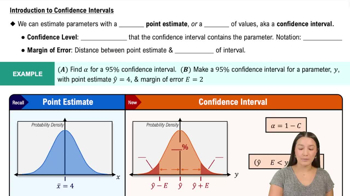
Confidence Interval

A confidence interval is a range of values, derived from sample statistics, that is likely to contain the true population parameter. It is calculated using the sample mean, standard deviation, and the critical value from the t-distribution, especially when the population standard deviations are unknown. In this context, it helps assess the difference in commuting times between the two bicycles.

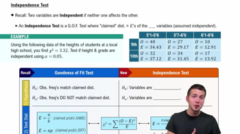
Independent Samples

Independent samples refer to two or more groups that are not related or paired in any way. In this scenario, the commuting times for the heavier and lighter bicycles are independent, meaning the performance of one does not affect the other. This independence is crucial for applying statistical tests that compare means, such as the t-test.

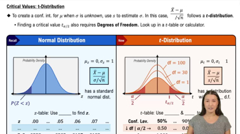
T-distribution

The t-distribution is a type of probability distribution that is symmetric and bell-shaped, similar to the normal distribution but with heavier tails. It is used in hypothesis testing and constructing confidence intervals when the sample size is small and the population standard deviation is unknown. In this case, the t-distribution will be used to calculate the confidence interval for the difference in commuting times.

Recommended video:

05:50

Critical Values: t-Distribution

Related Practice

Textbook Question

In Exercises 5–20, assume that the two samples are independent simple random samples selected from normally distributed populations, and do not assume that the population standard deviations are equal. (Note: Answers in Appendix D include technology answers based on Formula 9-1 along with “Table” answers based on Table A-3 with df equal to the smaller of n1-1 and n2-1)

Color and Cognition Researchers from the University of British Columbia conducted a study to investigate the effects of color on cognitive tasks. Words were displayed on a computer screen with background colors of red and blue. Results from scores on a test of word recall are given below. Higher scores correspond to greater word recall.

b. Construct a confidence interval appropriate for the hypothesis test in part (a). What is it about the confidence interval that causes us to reach the same conclusion from part (a)?

" style="max-width: 100%; white-space-collapse: preserve;" width="440">

views

Textbook Question

Second-Hand Smoke Samples from Data Set 15 “Passive and Active Smoke” include cotinine levels measured in a group of smokers ( n = 40, x_bar = 172.48 ng/mL, 119.50 ng/mL ) and a group of nonsmokers not exposed to tobacco smoke ( n = 40, x_bar = 16.35 ng/mL, 62.53 ng/mL ). Cotinine is a metabolite of nicotine, meaning that when nicotine is absorbed by the body, cotinine is produced.

b. The 40 cotinine measurements from the nonsmoking group consist of these values (all in ng/mL): 1, 1, 90, 244, 309, and 35 other values that are all 0. Does this sample appear to be from a normally distributed population? If not, how are the results from part (a) affected?

views

Textbook Question

In Exercises 5–16, use the listed paired sample data, and assume that the samples are simple random samples and that the differences have a distribution that is approximately normal.

The Freshman 15 The “Freshman 15” refers to the belief that college students gain 15 lb (or 6.8 kg) during their freshman year. Listed below are weights (kg) of randomly selected male college freshmen (from Data Set 13 “Freshman 15” in Appendix B). The weights were measured in September and later in April.

b. Construct the confidence interval that could be used for the hypothesis test described in part (a). What feature of the confidence interval leads to the same conclusion reached in part (a)?

105

views

Textbook Question

In Exercises 5–16, use the listed paired sample data, and assume that the samples are simple random samples and that the differences have a distribution that is approximately normal.

Measured and Reported Weights Listed below are measured and reported weights (lb) of random female subjects (from Data Set 4 “Measured and Reported” in Appendix B).

b. Construct the confidence interval that could be used for the hypothesis test described in part (a). What feature of the confidence interval leads to the same conclusion reached in part (a)?

121

views

Textbook Question

Better Tips by Giving Candy An experiment was conducted to determine whether giving candy to dining parties resulted in greater tips. The mean tip percentages and standard deviations are given below along with the sample sizes (based on data from “Sweetening the Till: The Use of Candy to Increase Restaurant Tipping,” by Strohmetz et al., Journal of Applied Social Psychology, Vol. 32, No. 2).

b. Construct the confidence interval suitable for testing the claim in part (a).

116

views

Textbook Question

Readability of Font On a Computer Screen The statistics shown below were obtained from a standard test of readability of fonts on a computer screen (based on data from “Reading on the Computer Screen: Does Font Type Have Effects on Web Text Readability?” by Ali et al., International Education Studies, Vol. 6, No. 3). Reading speed and accuracy were combined into a readability performance score (x), where a higher score represents better font readability.

b. Construct the confidence interval suitable for testing the claim in part (a).

106

views