Large Data Sets from Appendix B. In Exercises 21 and 22, use the data set in Appendix B. Assume that each sample is a simple random sample obtained from a population with a normal distribution.


Comparing Waiting Lines Refer to Data Set 30 “Queues” in Appendix B. Construct separate 95% confidence interval estimates of using the two-line wait times and the single-line wait times. Do the results support the expectation that the single line has less variation? Do the wait times from both line configurations satisfy the requirements for confidence interval estimates of sigma

Verified step by step guidance

1. Step 1: Identify the data set and variables. From the problem, we are working with Data Set 30 'Queues' in Appendix B. The two variables of interest are the wait times for the two-line configuration and the single-line configuration. These are the two groups for which we will construct separate 95% confidence intervals for the population standard deviation (σ).
2. Step 2: Verify the assumptions. The problem states that the samples are simple random samples and the population has a normal distribution. Confirm that the wait times for both configurations satisfy these assumptions by checking the data for normality (e.g., using a histogram, Q-Q plot, or a normality test like the Shapiro-Wilk test).
3. Step 3: Use the chi-square distribution to construct confidence intervals for the population standard deviation. The formula for the confidence interval of σ is: \( \left( \sqrt{\frac{(n-1)s^2}{\chi^2_{\alpha/2}}}, \sqrt{\frac{(n-1)s^2}{\chi^2_{1-\alpha/2}}} \right) \), where \( n \) is the sample size, \( s \) is the sample standard deviation, and \( \chi^2 \) are the critical values of the chi-square distribution with \( n-1 \) degrees of freedom.
4. Step 4: Calculate the sample standard deviation (s) for each group (two-line and single-line wait times) and determine the sample size (n). Use these values to compute the confidence intervals for each group using the formula from Step 3. Look up the critical chi-square values for a 95% confidence level and \( n-1 \) degrees of freedom.
5. Step 5: Compare the confidence intervals for the two groups. If the confidence interval for the single-line configuration is narrower (indicating less variation), this supports the expectation that the single line has less variation. Additionally, confirm that the wait times satisfy the requirements for confidence interval estimates of σ by ensuring the data is approximately normal and the sample sizes are sufficient.

Key Concepts

Confidence Interval

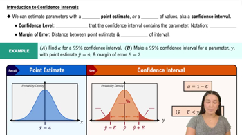
A confidence interval is a range of values, derived from sample statistics, that is likely to contain the true population parameter with a specified level of confidence, typically 95%. It provides an estimate of uncertainty around a sample mean or proportion, allowing researchers to infer about the population. The width of the interval reflects the variability in the data and the sample size, with larger samples generally yielding narrower intervals.

Variation and Standard Deviation

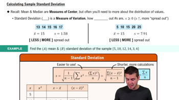
Variation refers to how much data points in a set differ from each other and from the mean. Standard deviation is a key measure of this variation, quantifying the average distance of each data point from the mean. In the context of waiting times, lower variation indicates more consistent wait times, which is crucial for comparing different queue configurations, such as single-line versus two-line systems.

Normal Distribution

A normal distribution is a probability distribution that is symmetric about the mean, showing that data near the mean are more frequent in occurrence than data far from the mean. Many statistical methods, including confidence intervals, assume that the underlying data follows a normal distribution. This assumption is important when analyzing wait times, as it affects the validity of the confidence intervals constructed from the sample data.