The Lineweaver-Burk plot is a graphical representation used in enzyme kinetics to illustrate the relationship between the reciprocal of the reaction velocity (V) and the reciprocal of the substrate concentration (S). The equation for this plot can be derived from the linear equation of a line, y = mx + b, where m represents the slope and b the y-intercept. In the context of enzyme kinetics, the Lineweaver-Burk equation can be expressed as:
\[\frac{1}{V} = \frac{K_m}{V_{max}} \cdot \frac{1}{[S]} + \frac{1}{V_{max}}\]
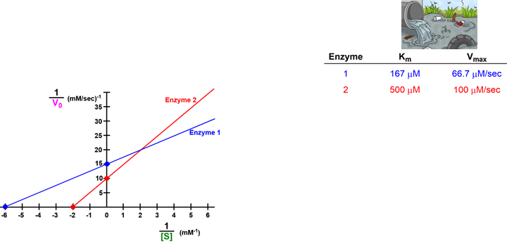
Here, Km is the Michaelis constant, and Vmax is the maximum reaction velocity. The slope of the line, m, is defined as the ratio of Km to Vmax, while the y-intercept, b, is the reciprocal of Vmax.
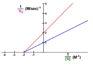
Understanding how to shift the line on a Lineweaver-Burk plot involves manipulating these two parameters: the slope and the y-intercept. A slope of zero indicates a horizontal line, which is not possible in enzyme kinetics since the slope, defined as Km/Vmax, must always be positive. As the slope increases, the line becomes steeper, indicating a higher ratio of Km to Vmax.
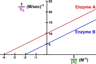
For example, if the slope increases from 1 to 2 or 3, the steepness of the line will correspondingly increase. The y-intercept, on the other hand, represents the point where the line crosses the y-axis, which is influenced by the value of Vmax. An increase in the y-intercept elevates the line's position on the y-axis, indicating a lower Vmax.
It is crucial to note that the slope of a Lineweaver-Burk plot cannot be zero or negative, ensuring that all lines will have a positive slope. This characteristic simplifies the interpretation of the plot, as it eliminates the possibility of horizontal or downward-sloping lines. In summary, the Lineweaver-Burk plot serves as a valuable tool in enzyme kinetics, allowing for the visualization and analysis of key parameters such as Km and Vmax through the manipulation of slope and y-intercept.