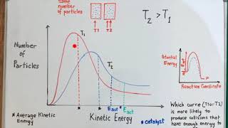
00:346.1 Sketch and Explain the Maxwell-Boltzmann Energy Distribution Curve [SL IB Chemistry]Richard Thornley605views
04:09Maxwell–Boltzmann Distribution Curves | Revision for Chemistry A-LevelScience and Maths by Primrose Kitten285views
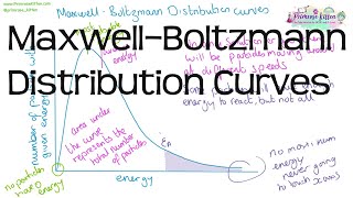
02:41The Maxwell Boltzmann Distribution - A-level Chemistry [❗VIDEO UPDATED - LINK IN DESCRIPTION👇]SnapRevise536views
05:17Kinetic Energy (Maxwell-Boltzmann) Distribution Curves Examples and Practice ProblemsConquer Chemistry670views

 00:54
00:54

![6.1 Sketch and Explain the Maxwell-Boltzmann Energy Distribution Curve [SL IB Chemistry]](https://img.youtube.com/vi/YnHIfqUZi48/mqdefault.jpg)


![The Maxwell Boltzmann Distribution - A-level Chemistry [❗VIDEO UPDATED - LINK IN DESCRIPTION👇]](https://img.youtube.com/vi/SGCynIaOr6A/mqdefault.jpg)