Dilutions: Videos & Practice Problems

A stock solution is a concentrated solution that can be diluted by adding more solvent, typically water, to achieve a lower concentration. The dilution process can be expressed with the equation $m_1{v}_1=m_2{v}_2$, where m1 and v1 are the molarity and volume before dilution, and m2 and v2 are after dilution. This highlights the transition from a higher to a lower molarity solution.

Solution Dilution Process

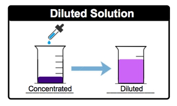
A stock solution is a concentrated solution that can be diluted for various laboratory applications. Dilution involves adding more solvent, typically water, to a solution to decrease its concentration. For instance, when a dark purple solution, which indicates a high concentration, is gradually mixed with water, the color lightens to a fuchsia hue. This visual change signifies that the solution has become less concentrated. In summary, dilutions are achieved by adding water to the original solution, resulting in a diluted solution with a lower concentration.

Ranking Solutions Example

In this scenario, we are tasked with arranging solutions based on their molarity, which is defined as the number of moles of solute per liter of solution. Molarity (M) can be calculated using the formula:

M = \frac{n}{V}

where n is the number of moles of solute and V is the volume of the solution in liters.

Let's analyze the provided solutions:

For solution A, there are 5 spheres representing 5 moles of solute in 1 liter of solution. Thus, the molarity is:

M_A = \frac{5 \text{ moles}}{1 \text{ L}} = 5 \text{ M}

For solution B, there are 3 spheres, indicating 3 moles of solute in 2 liters of solution. Therefore, the molarity is:

M_B = \frac{3 \text{ moles}}{2 \text{ L}} = 1.5 \text{ M}

For solution C, there are 6 spheres, which means 6 moles of solute in 3 liters of solution. The molarity is calculated as:

M_C = \frac{6 \text{ moles}}{3 \text{ L}} = 2 \text{ M}

Now, to arrange the solutions from least concentrated to most concentrated based on their molarity, we find:

1. Solution B: 1.5 M

2. Solution C: 2 M

3. Solution A: 5 M

Thus, the order from least concentrated to most concentrated is B, C, and A.

Dilution Equation

Understanding dilution is essential in chemistry, as it allows us to create solutions with lower concentrations from more concentrated ones. The process of dilution can be quantitatively described using the equation:

\( M_1 V_1 = M_2 V_2 \)

In this equation, \( M_1 \) and \( V_1 \) represent the molarity and volume of the solution before dilution, while \( M_2 \) and \( V_2 \) represent the molarity and volume after dilution. It is important to note that \( M_1 \), the molarity of the concentrated solution, is always greater than \( M_2 \), the molarity of the diluted solution.

The final volume after dilution, \( V_2 \), is determined by the initial volume \( V_1 \) plus the volume of solvent added. This relationship can be expressed as:

\( V_2 = V_1 + V_{\text{solvent}} \)

By applying these principles, one can effectively prepare solutions with desired concentrations, which is a fundamental skill in various scientific applications.

Dilution Calculation Example

To determine the volume of a concentrated solution needed to prepare a diluted solution, we can apply the concept of dilution, which involves a single compound with two different molarities. In this case, we are working with hydrobromic acid (HBr) and using the dilution equation:

M₁V₁ = M₂V₂

Here, M₁ represents the molarity of the concentrated solution, while M₂ is the molarity of the diluted solution. V₁ is the volume of the concentrated solution we need to find, and V₂ is the volume of the diluted solution.

In this example, we have:

• M₁ = 5.2 M (the concentrated solution)
• M₂ = 2.7 M (the diluted solution)
• V₂ = 3.5 L (the volume of the diluted solution)

Since we are looking for V₁, we can rearrange the equation:

V₁ = (M₂V₂) / M₁

Substituting the known values:

V₁ = (2.7 M × 3.5 L) / 5.2 M

Calculating this gives:

V₁ = 1.8173 L

To convert this volume into milliliters, we use the conversion factor where 1 L = 1000 mL:

V₁ = 1.8173 L × 1000 mL/L = 1817.3 mL

Considering significant figures, since the values 5.2, 3.5, and 2.7 all have two significant figures, we round our final answer to:

V₁ = 1800 mL

This example illustrates that when dealing with a single compound and two different molarities, we can effectively use the dilution formula to find the required volume of the concentrated solution.

To what final volume would 100 mL of 5.0 M KCl have to be diluted in order to make a solution that is 0.54 M KCl?

• A. 72 mL
• B. 289 mL
• C. 330 mL
• D. 930 mL
• E. 1400 mL

Answer: (D)

If 880 mL of water is added to 125.0 mL of a 0.770 M HBrO₄ solution what is the resulting molarity?

• A. 0.096 M
• B. 0.136 M
• C. 0.257 M
• D. 0.892 M
• E. 1.76 M

Answer: (A)

A student prepared a stock solution by dissolving 25.00 g of NaOH in enough water to make 150.0 mL solution. The student took 20.0 mL of the stock solution and diluted it with enough water to make 250.0 mL solution. Finally taking 75.0 mL of that solution and dissolving it in water to make 500 mL solution. What is the concentration of NaOH for this final solution? (MW of NaOH:40.00 g/mol).

• A. 0.0500 M
• B. 0.025 M
• C. 0.005 M
• D. 0.500 M
• E. 0.0100 M

Answer: (A)

Here’s what students ask on this topic:

What is the purpose of performing a dilution in chemistry?

The purpose of performing a dilution in chemistry is to decrease the concentration of a solution by adding more solvent, typically water. This is often done to prepare solutions with specific, lower concentrations for use in experiments or analytical procedures. Dilutions are essential for ensuring accurate and reproducible results in the laboratory, as working with overly concentrated solutions can lead to errors or undesired reactions. By diluting a stock solution, chemists can achieve the desired molarity for their experiments while maintaining precision and control over the solution's properties.

How do you calculate the final concentration of a solution after dilution?

The final concentration of a solution after dilution can be calculated using the dilution equation:

$M_1{V}_1=M_2{V}_2$

Here, $M_1$ and $V_1$ are the molarity and volume of the concentrated solution before dilution, while $M_2$ and $V_2$ are the molarity and volume after dilution. Rearrange the equation to solve for the unknown, such as $M_2$, if needed. This equation ensures that the number of moles of solute remains constant before and after dilution.

What is the difference between a stock solution and a diluted solution?

A stock solution is a concentrated solution that contains a high amount of solute per unit volume. It is typically prepared in advance and used as a starting point for creating solutions of lower concentrations. A diluted solution, on the other hand, is created by adding a solvent, usually water, to the stock solution to decrease its concentration. The diluted solution has a lower molarity compared to the stock solution, as the solute is spread out over a larger volume. This process allows chemists to prepare solutions with precise concentrations for specific experimental needs.

How does the color of a solution change during dilution?

During dilution, the color of a solution typically becomes lighter or less intense. This change occurs because the concentration of the solute, which is responsible for the solution's color, decreases as more solvent is added. For example, a dark purple solution may turn into a lighter purple or fuchsia as it is diluted. The color change visually indicates that the solution's concentration has been reduced, although the exact appearance depends on the solute's properties and concentration.

What does the equation M1V1 = M2V2 represent in the context of dilutions?

The equation $M_1{V}_1=M_2{V}_2$ represents the relationship between the concentration and volume of a solution before and after dilution. Here, $M_1$ and $V_1$ are the molarity and volume of the concentrated solution, while $M_2$ and $V_2$ are the molarity and volume after dilution. This equation ensures that the number of moles of solute remains constant during the dilution process, as the solute is not removed, only spread out over a larger volume.

How do you determine the volume of solvent added during a dilution?

The volume of solvent added during a dilution can be determined by subtracting the initial volume of the solution ($V_1$) from the final volume of the solution ($V_2$). The formula is:

$V_{\mathrm{solvent}}=V_2-V_1$

Here, $V_{\mathrm{solvent}}$ is the volume of solvent added. This calculation is useful for determining how much solvent is needed to achieve the desired final concentration and volume of the solution.